library(network)
library(ergm)
library(sna)
library(Bergm)
set.seed(42)
We adopt the notation and syntax of the official Statnet ERGM workshop tutorial. More details on syntax, troubleshooting, etc are documented there and in the documentation. Below, we “borrow” an example from the tutorial and expand on the math/stats/theory quite a bit.
Faux Mesa High
We will use a simulated mutual friendship network of a faux high school from the ergm package. There are 205 students (nodes) and 203 reported friendships (edges). Vertex attributes include Grade, Race, and Sex. Our substantive question: what explains friendship ties at this school? Is it just the overall density of edges, or do some groups (e.g. grade, race, sex) have more friendships overall (activity)? Do some groups form ties disproportionately within themselves (homophily)?
data(faux.mesa.high)
mesa <- faux.mesa.high
mesa
Network attributes:
vertices = 205
directed = FALSE
hyper = FALSE
loops = FALSE
multiple = FALSE
bipartite = FALSE
total edges= 203
missing edges= 0
non-missing edges= 203
Vertex attribute names:
Grade Race Sex
No edge attributesplot(mesa, vertex.col = "Grade")
legend("bottomleft", fill = 7:12,
legend = paste("Grade", 7:12))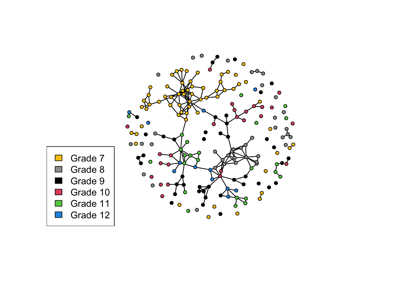
We cannot apply the usual statistical tests (e.g. regression) since those require independent observations, and intuitively we know that network ties are not independent (e.g., my own friends are likely to be friends with each other—this alone interlocks the entire network). Instead, we view the observed network as one possible realization of real social processes subject to stochastic noise, and we aim to infer a distribution of plausible realizations under those processes. Unlike “standard” inference in which we infer properties about a population based on a sample, we are using our full population (or at least a snapshot of it) to infer a “distribution of alternate realities.”
We might like to consider the distribution of all graphs with properties similar to the observed network, like number of edges or triangles, etc, where “more similar = more likely”, but enumeration of this set would be impossible (e.g., there are about \(10^{500}\) ways to assign exactly 203 friendships to 205 students, as compared to about \(10^{80}\) atoms in the universe, before even considering slight deviations like \(\pm1, \pm2, \ldots\) friendships). Instead, we use a process which generates random graphs that are representative of this distribution.
ERGMs
Informal “Derivation”
Let \(Y\) be the random variable which represents our theoretical distribution of networks. Let’s image that the probability of network \(y\) depends on two things:
- \(g_1(y)\): the number of edges in \(y\)
- \(g_2(y)\): the number of triangles in \(y\)
We might naively try to fit the probability as linear, \[\theta_1g_1(y) + \theta_2g_2(y),\] but this is clearly problematic since it can take both positive and negative values (e.g., if we want to penalize triangles then \(\theta_2<0\)). Instead, we fit the (unnormaliezd) log-probability as linear, meaning
\[\Pr(Y=y) \;\propto\; \exp\{\theta_1g_1(y) + \theta_2g_2(y)\}.\] To get true probabilities, we normalize: \[\Pr(Y=y) \;=\; \frac{\exp\{\theta_1g_1(y) + \theta_2g_2(y)\}}{\sum_{y'}\exp\{\theta_1g_1(y') + \theta_2g_2(y')\}}.\]
Formal ERGM Model
Generalizing, an (unweighted) exponential random graph model (ERGM) assign probabilities
\[ \Pr(Y=y) = \frac{\exp\{\theta^\top g(y)\}}{k(\theta)}, \qquad k(\theta) = \sum_{y'} \exp\{\theta^\top g(y')\}, \]
where \(g(y) = (g_1(y), \ldots, g_p(y))^\top\) is a vector of sufficient statistics (usually counts of structural features) and \(\theta=(\theta_1, \ldots, \theta_p)^\top\) is the parameter vector. Notably, \(k(\theta)\) is typically impossible to compute, since the sum over \(y'\) is intractable.
A fairly technical theorem by Hammersley and Clifford states, loosely, that many network models can be expressed in such form.
Interpretation of model parameters
Let \(y_{-ij}\) denote an arbitrary but fixed network with the value of edge \(ij\) left unspecified.
- \(y^+\) is defined as \(y_{-ij}\) with \(y_{ij}=1\), and
- \(y^-\) is defined as \(y_{-ij}\) with \(y_{ij}=0\).
Define the change statistic as \[\delta_{ij}(y):= g(y^+)-g(y^-).\]
Importantly, we can divide probabilities in the formula above (and cancel the intractable \(k(\theta)\) term!) and derive
\[\log \frac{\Pr(Y=y^+)}{\Pr(Y=y^-)} = \operatorname{logit} \Pr(Y_{ij}=1|Y_{-ij}=y_{-ij}) = \theta^\top \delta_{ij}(y) = \sum\theta_k\{g_k(y^+)-g_k(y^-)\},\]
which closely resembles the interpretation of coefficients in logistic regression. The biggest difference is the logit function now represents conditional log-odds of an edge holding the rest of the network fixed; notably, we typically cannot say we are holding the other covariates fixed, since changing one edge may change several covariates.
For example, suppose as before that \[\Pr(Y=y) \;=\; \frac{\exp\{\theta_1g_1(y) + \theta_2g_2(y)\}}{\sum_{y'}\exp\{\theta_1g_1(y') + \theta_2g_2(y')\}},\] where \(g_1\), \(g_2\) count edges and triangles. Then \[\operatorname{logit} \Pr(Y_{ij}=1|Y_{-ij}=y_{-ij}) = \theta^\top \delta_{ij}(y) = \theta_1 \cdot 1 + \theta_2\cdot \#(\text{shared partners}),\] since adding the edge \(ij\) will create a triangle for every vertex \(k\) such that \(ik\) and \(jk\) are already edges. The conditional log-odds change depending on network structure!
Implementing ERGMs
We will fit three ERGMs on our data. Model 1 uses edges only and acts as a baseline. Model 2 follows the Statnet tutorial and further includes grade and race activity and homophily. After considering GOF for these models we will discuss Model 3, which includes triadic closure, but more on that later.
edges: total number of ties; controls overall density.nodefactor("Grade")/nodefactor("Race"): differential activity; nodes in certain grades or racial groups may tend to have more (or fewer) friendshipsnodematch("Grade", diff = TRUE)/nodematch("Race", diff = TRUE): differential homophily; nodes in certain grades or racial groups may tend to prefer within-group friendships; thediff = TRUEoption allows for different propensities for within-group ties at each level of the attribute, rather than a shared homophily coefficient.
Models 1 and 2 include only dyad-independent terms; that is, for each pair \((i,j)\), the change statistics \(\delta_{ij}(y)\) depend only on nodes \(i\) and \(j\) (not who they are connected to). By default, ergm() targets maximum likelihood (MLE): it chooses \(\hat\theta\) to make the observed network \(y_{\text{obs}}\) as probable as possible under the model; i.e., \[ \hat{\theta} = \operatorname{argmax}_{\theta} \Pr(Y=y_{\text{obs}} \mid \theta).\] The details do not matter here, but we will need to pay attention to what algorithm(s) are being employed later for diagnostics. We’ll use default settings; see documentation for more options.
Model 1: edges only
fauxmodel.01 <- ergm(mesa ~ edges)
summary(fauxmodel.01)
Call:
ergm(formula = mesa ~ edges)
Maximum Likelihood Results:
Estimate Std. Error MCMC % z value Pr(>|z|)
edges -4.62502 0.07053 0 -65.58 <1e-04 ***
---
Signif. codes: 0 '***' 0.001 '**' 0.01 '*' 0.05 '.' 0.1 ' ' 1
Null Deviance: 28987 on 20910 degrees of freedom
Residual Deviance: 2286 on 20909 degrees of freedom
AIC: 2288 BIC: 2296 (Smaller is better. MC Std. Err. = 0)This model matches total tie count only and ignores grade and race structure. Notice that the edges estimate is strongly negative since the network is relatively sparse. Because there is no dependence on other edges in this model, the (conditional) probability of any edge is \[\Pr(Y_{ij}=1)=\Pr(Y_{ij}=1 |Y_{-ij}=y_{-ij}) = \operatorname{logit}^{-1}(-4.62502)\simeq 0.0097,\] so every edge has a the same \(0.97\%\) chance of existing. (One can show that an Erds–R'enyi model with parameter \(p\) is equivalent to an edges-only ERGM with paremter \(\theta=\operatorname{logit}(p)\).)
Model 2: grade and race activity and homophily
fauxmodel.02 <- ergm(mesa ~ edges +
  nodefactor("Grade") + nodematch("Grade", diff = TRUE) +
  nodefactor("Race") + nodematch("Race", diff = TRUE))
summary(fauxmodel.02)
Call:
ergm(formula = mesa ~ edges + nodefactor("Grade") + nodematch("Grade",
diff = TRUE) + nodefactor("Race") + nodematch("Race", diff = TRUE))
Maximum Likelihood Results:
Estimate Std. Error MCMC % z value Pr(>|z|)
edges -8.0538 1.2561 0 -6.412 < 1e-04 ***
nodefactor.Grade.8 1.5201 0.6858 0 2.216 0.026663 *
nodefactor.Grade.9 2.5284 0.6493 0 3.894 < 1e-04 ***
nodefactor.Grade.10 2.8652 0.6512 0 4.400 < 1e-04 ***
nodefactor.Grade.11 2.6291 0.6563 0 4.006 < 1e-04 ***
nodefactor.Grade.12 3.4629 0.6566 0 5.274 < 1e-04 ***
nodematch.Grade.7 7.4662 1.1730 0 6.365 < 1e-04 ***
nodematch.Grade.8 4.2882 0.7150 0 5.997 < 1e-04 ***
nodematch.Grade.9 2.0371 0.5538 0 3.678 0.000235 ***
nodematch.Grade.10 1.2489 0.6233 0 2.004 0.045111 *
nodematch.Grade.11 2.4521 0.6124 0 4.004 < 1e-04 ***
nodematch.Grade.12 1.2987 0.6981 0 1.860 0.062824 .
nodefactor.Race.Hisp -1.6659 0.2963 0 -5.622 < 1e-04 ***
nodefactor.Race.NatAm -1.4725 0.2869 0 -5.132 < 1e-04 ***
nodefactor.Race.Other -2.9618 1.0372 0 -2.856 0.004296 **
nodefactor.Race.White -0.8488 0.2958 0 -2.869 0.004112 **
nodematch.Race.Black -Inf 0.0000 0 -Inf < 1e-04 ***
nodematch.Race.Hisp 0.6912 0.3451 0 2.003 0.045153 *
nodematch.Race.NatAm 1.2482 0.3550 0 3.517 0.000437 ***
nodematch.Race.Other -Inf 0.0000 0 -Inf < 1e-04 ***
nodematch.Race.White 0.3140 0.6405 0 0.490 0.623947
---
Signif. codes: 0 '***' 0.001 '**' 0.01 '*' 0.05 '.' 0.1 ' ' 1
Null Deviance: 28987 on 20910 degrees of freedom
Residual Deviance: 1798 on 20889 degrees of freedom
AIC: 1836 BIC: 1987 (Smaller is better. MC Std. Err. = 0)
Warnings:
* The following terms have infinite coefficient estimates due to an
extreme sufficient statistic:
nodematch.Race.Black, nodematch.Race.OtherThe -Inf values are the result of a boundary problem. The possible values of \(g(y)\) exist in a vector space. If the observed statistics vector \(g(y_{\text{obs}})\) lies on or close to the boundary convex hull of the feasible statistics, the MLE may not exist or may be unstable. It’s easy to see why it failed here by looking at the original data.
table(mesa %v% "Race")
Black  Hisp NatAm Other White
6 109 68 4 18 mixingmatrix(mesa, "Race") Black Hisp NatAm Other White
Black 0 8 13 0 5
Hisp 8 53 41 1 22
NatAm 13 41 46 0 10
Other 0 1 0 0 0
White 5 22 10 0 4There are only six Black students and four in the Other category in the original data, and the mixing matrix shows no within-group ties for those races. Hence the “infinite penalty.”
Goodness of fit
We used our single observed network \(y_{\text{obs}}\) to return point estimates \(\hat\theta\). We now ask whether networks simulated by parameters \(\hat\theta\) resemble \(y_{\text{obs}}\) on features beyond those explicitly forced by the fit. Internally, gof() uses Markov Chain Monte Carlo (MCMC) to simulate random graphs at the given \(\hat\theta\).
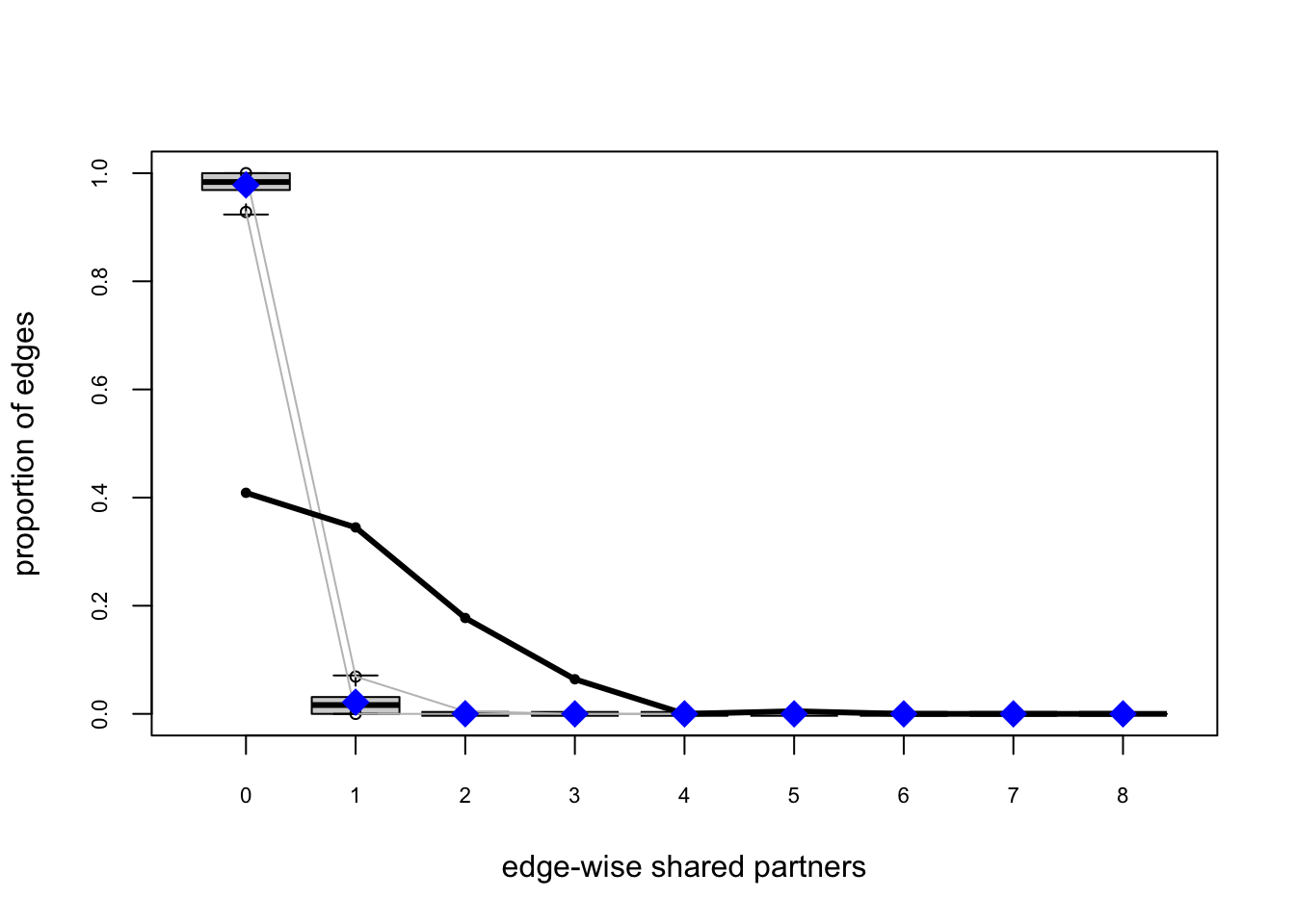
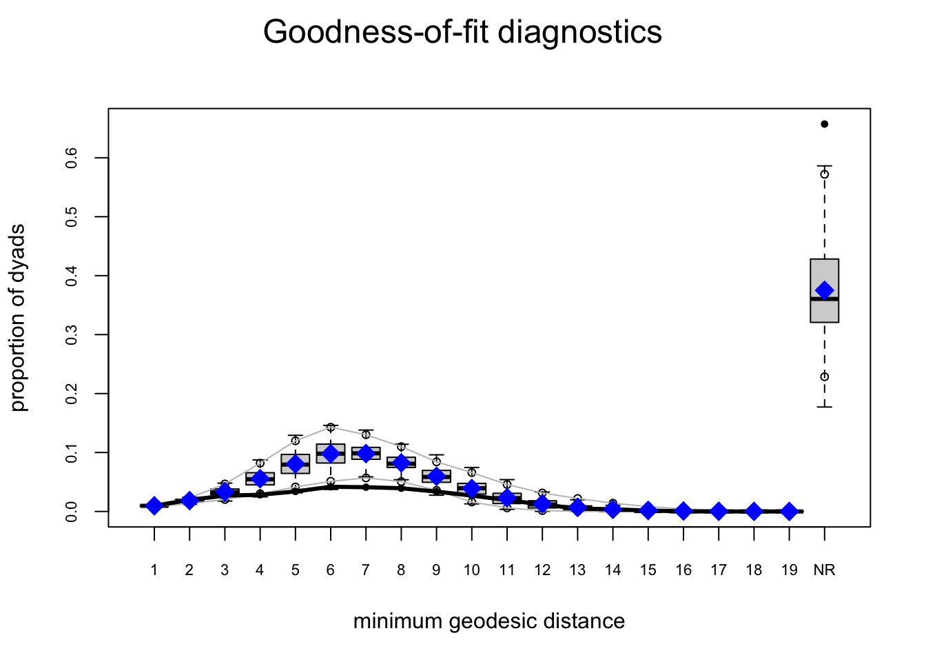
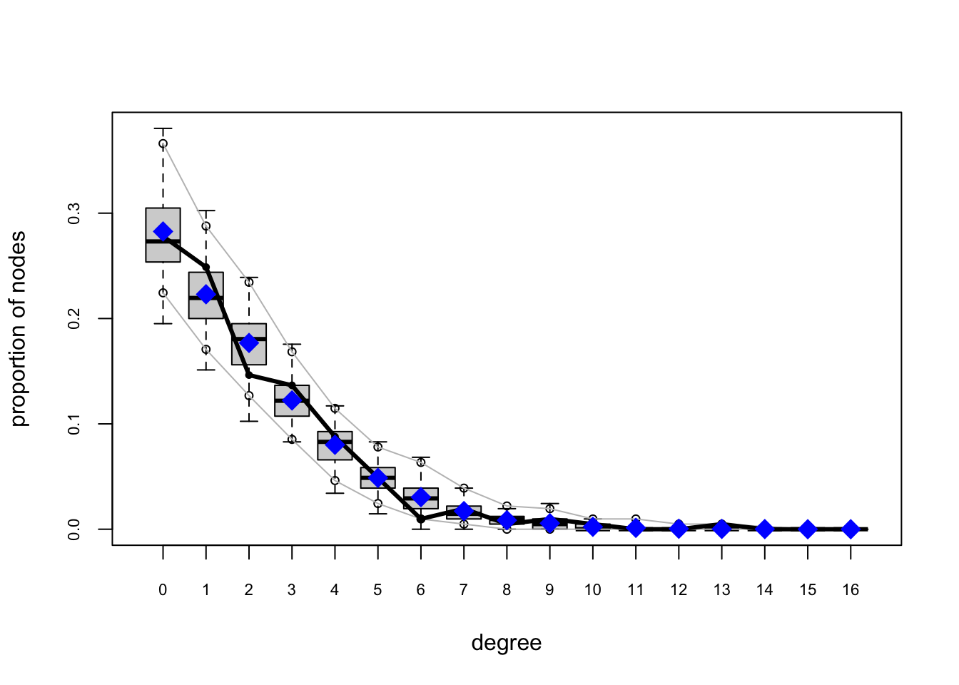
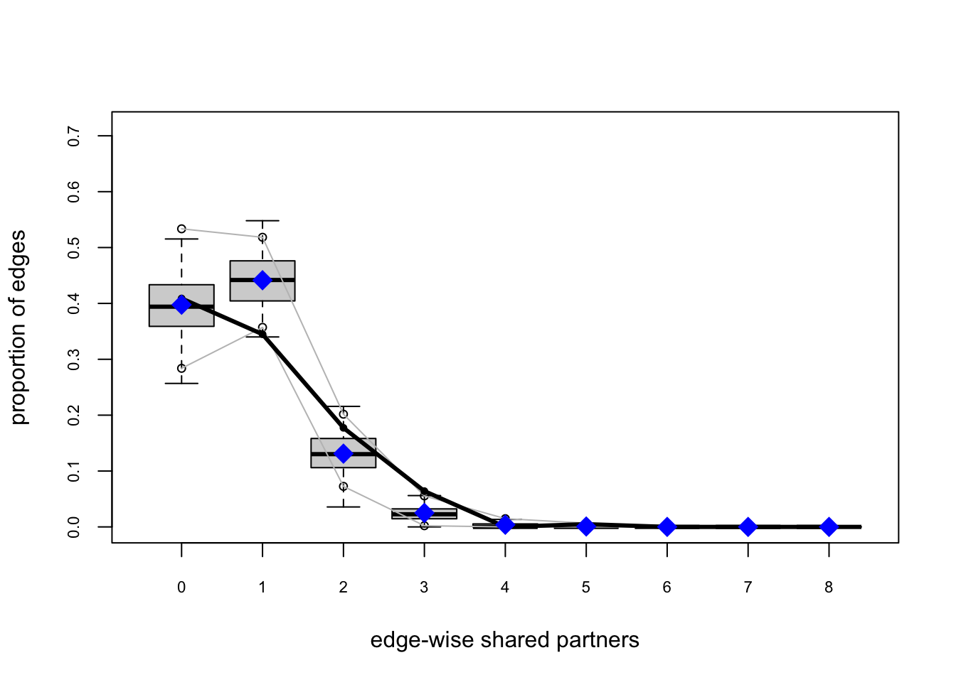
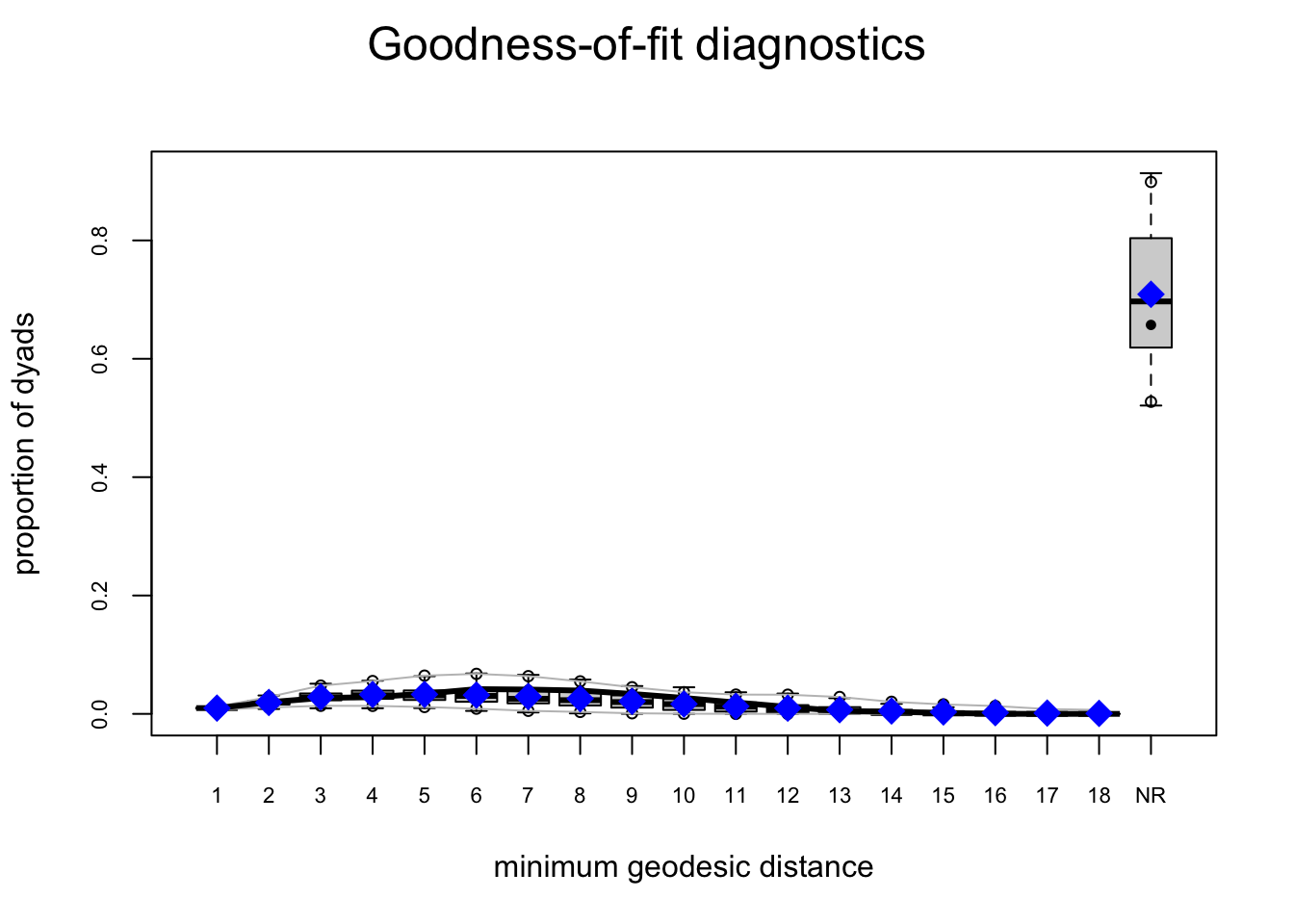
For Model 1 (edges only), GOF is predictably poor. We call gof() to simulate networks at \(\hat\theta\) and compare observed versus simulated distributions for degree, edgewise shared partners, and minimum geodesic distance. The solid lines marks \(y_{\text{obs}}\); box-plots summarize the simulations.
fauxmodel.01.gof <- gof(fauxmodel.01)
plot(fauxmodel.01.gof)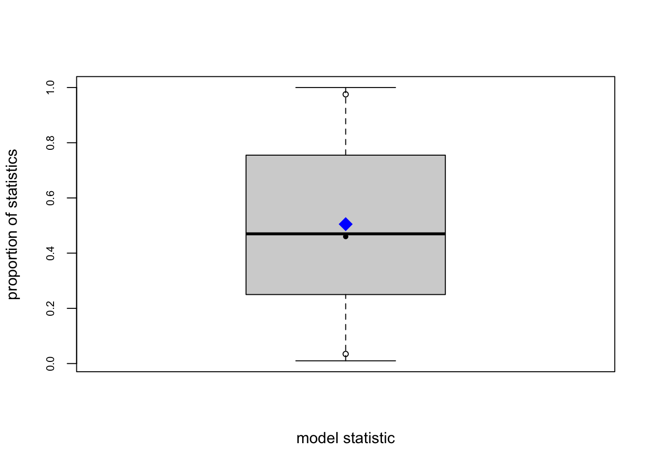
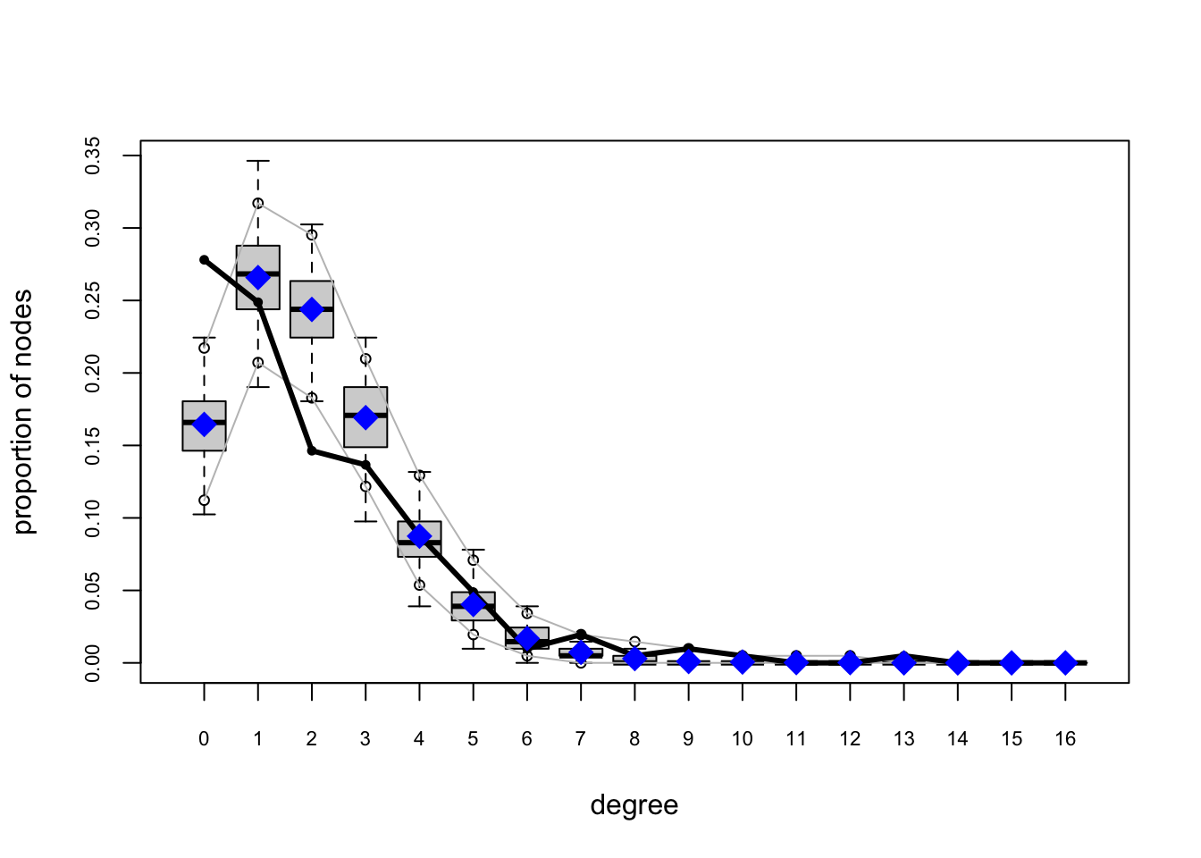
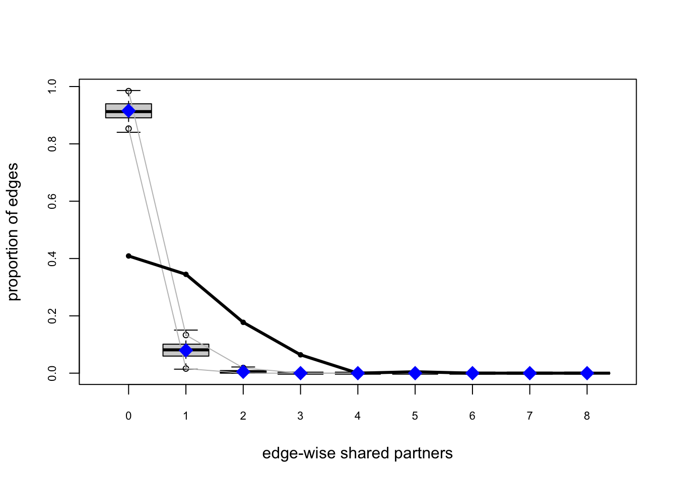
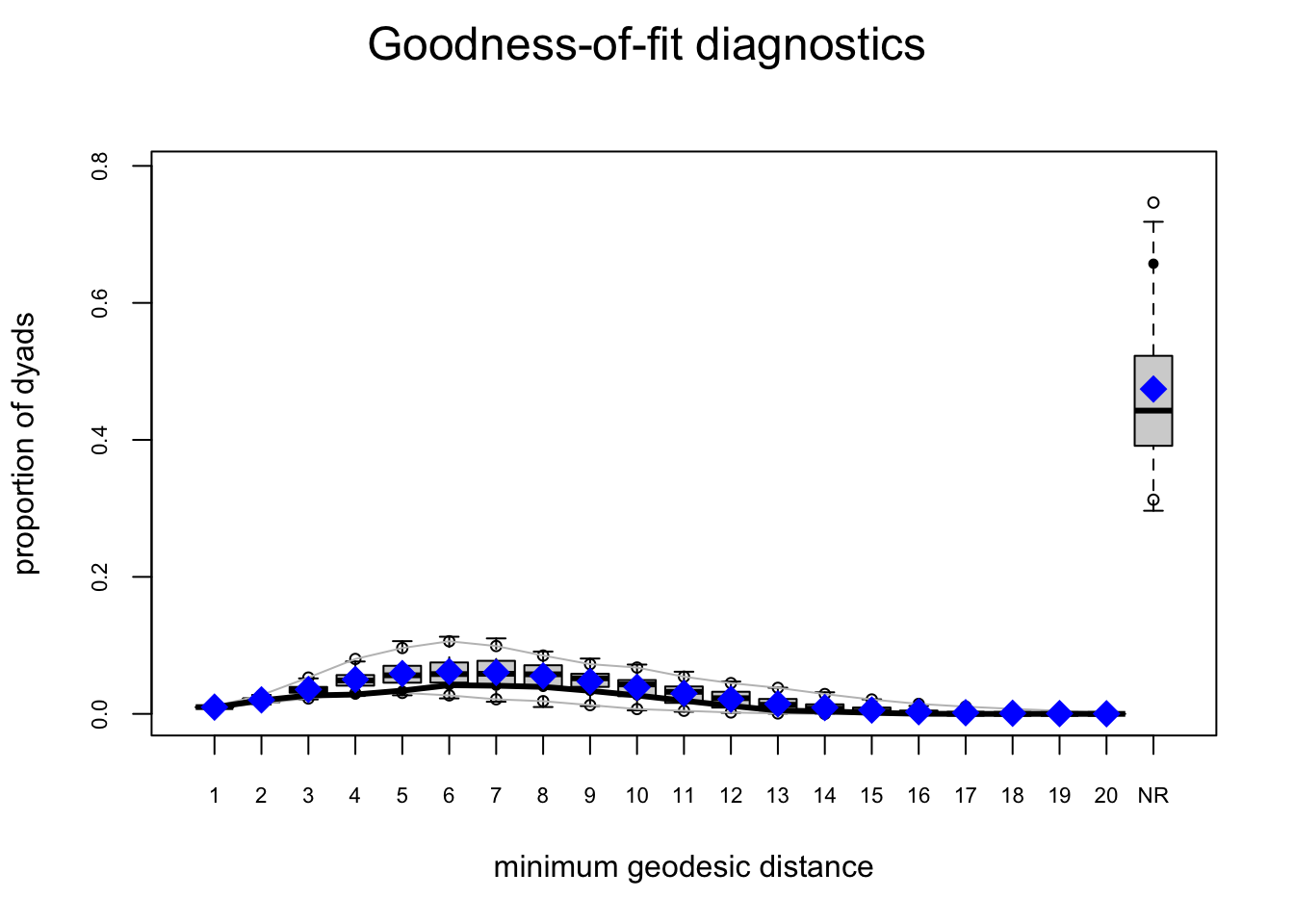
For Model 2, we have improvement but still not great.
fauxmodel.02.gof <- gof(fauxmodel.02)
plot(fauxmodel.02.gof)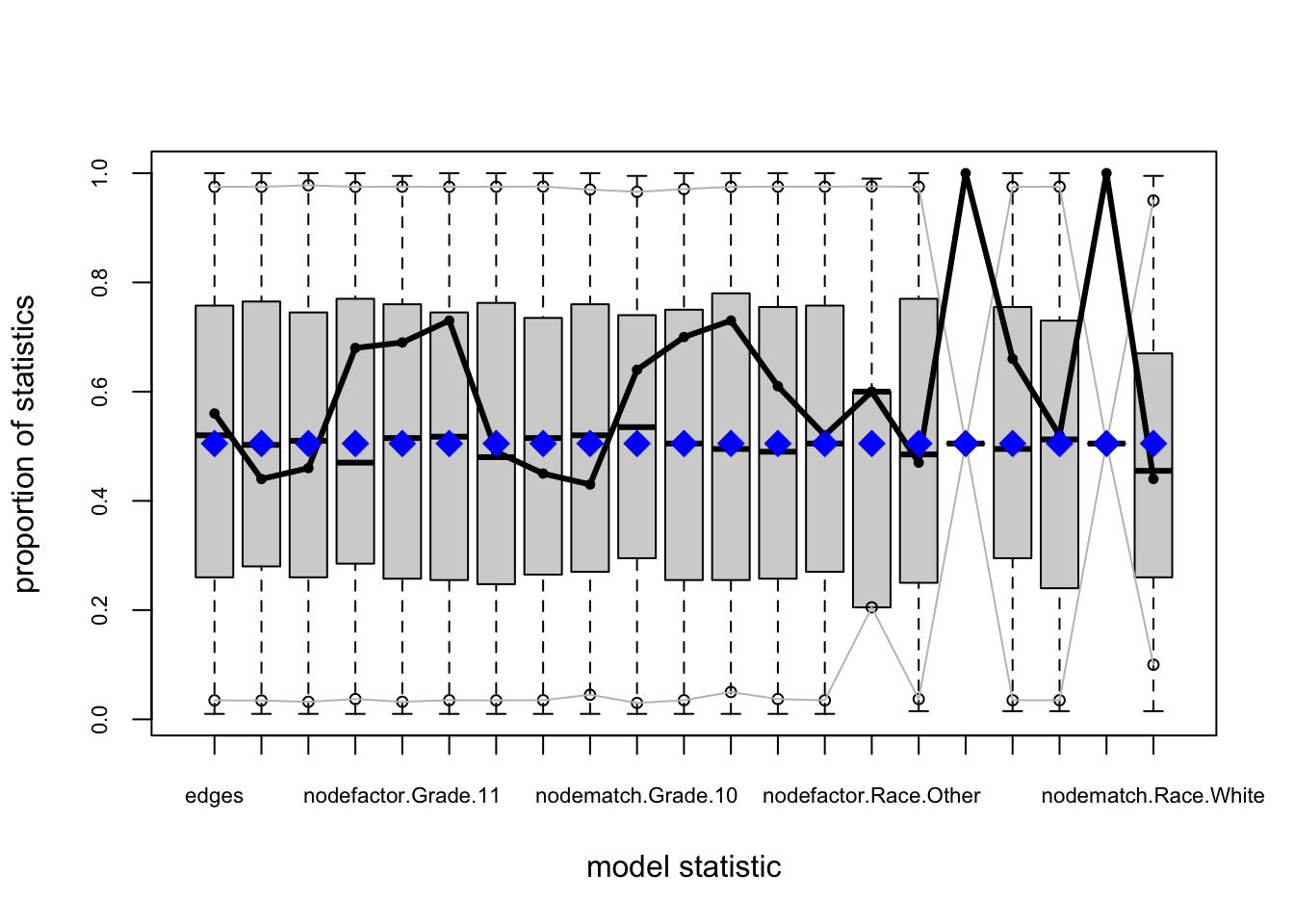
Model 3: Adding triadic closure
Homophily and activity terms do not describe structural clustering: if \(i\) is friends with \(j\), and \(j\) is friends with \(k\), then \(i\) and \(k\) are more likely to become friends (triadic closure).
We could add the raw triangle count as a sufficient statistic, but this is known to often cause degeneracy (probability mass collapses, and the ERGM places most of its probability on unrealistic networks, like nearly empty or nearly complete graphs). Instead, the geometrically weighted edgewise shared partners gwesp is the standard way to reward ties between pairs who share mutual friends. We will use
gwesp(0.25, fixed = TRUE)
which specifies a fixed decay parameter of 0.25: going from 0 to 1 shared partners matters a lot, going from 1 to 2 shared partners adds a little more value, and every additional partner beyond continuse this diminishing return of value added. A decay parameters closer to 0 means a steeper / more extreme diminishing return curve.
fauxmodel.03 <- ergm(mesa ~ edges +
  nodefactor("Grade") + nodematch("Grade", diff = TRUE) +
  nodefactor("Race") + nodematch("Race", diff = TRUE) +
  gwesp(0.25, fixed = TRUE))
summary(fauxmodel.03)
Call:
ergm(formula = mesa ~ edges + nodefactor("Grade") + nodematch("Grade",
diff = TRUE) + nodefactor("Race") + nodematch("Race", diff = TRUE) +
gwesp(0.25, fixed = TRUE))
Monte Carlo Maximum Likelihood Results:
Estimate Std. Error MCMC % z value Pr(>|z|)
edges -8.5193 1.1948 0 -7.130 < 1e-04 ***
nodefactor.Grade.8 1.3958 0.6609 0 2.112 0.034690 *
nodefactor.Grade.9 2.1613 0.6271 0 3.446 0.000568 ***
nodefactor.Grade.10 2.4687 0.6288 0 3.926 < 1e-04 ***
nodefactor.Grade.11 2.2418 0.6305 0 3.555 0.000377 ***
nodefactor.Grade.12 2.8643 0.6231 0 4.597 < 1e-04 ***
nodematch.Grade.7 5.9567 1.1606 0 5.132 < 1e-04 ***
nodematch.Grade.8 3.2186 0.6571 0 4.898 < 1e-04 ***
nodematch.Grade.9 1.6306 0.4737 0 3.442 0.000577 ***
nodematch.Grade.10 1.0672 0.5560 0 1.919 0.054957 .
nodematch.Grade.11 1.8177 0.5288 0 3.437 0.000588 ***
nodematch.Grade.12 0.9525 0.5846 0 1.629 0.103251
nodefactor.Race.Hisp -1.1029 0.2490 0 -4.429 < 1e-04 ***
nodefactor.Race.NatAm -1.0893 0.2473 0 -4.405 < 1e-04 ***
nodefactor.Race.Other -2.1035 0.9797 0 -2.147 0.031780 *
nodefactor.Race.White -0.5921 0.2494 0 -2.374 0.017579 *
nodematch.Race.Black -Inf 0.0000 0 -Inf < 1e-04 ***
nodematch.Race.Hisp 0.5578 0.3033 0 1.839 0.065928 .
nodematch.Race.NatAm 1.0711 0.3080 0 3.477 0.000506 ***
nodematch.Race.Other -Inf 0.0000 0 -Inf < 1e-04 ***
nodematch.Race.White 0.3163 0.6197 0 0.510 0.609794
gwesp.fixed.0.25 1.4037 0.1124 0 12.486 < 1e-04 ***
---
Signif. codes: 0 '***' 0.001 '**' 0.01 '*' 0.05 '.' 0.1 ' ' 1
Null Deviance: 28987 on 20910 degrees of freedom
Residual Deviance: 1624 on 20888 degrees of freedom
AIC: 1664 BIC: 1823 (Smaller is better. MC Std. Err. = 0.4307)
Warnings:
* The following terms have infinite coefficient estimates due to an
extreme sufficient statistic:
nodematch.Race.Black, nodematch.Race.OtherEstimation with MCMLE
Because gwesp is dyad-dependent (the change statistic \(\delta_{ij}(y)\) depends on shared partners elsewhere in the graph), the MLE algorithm used for dyad-independent Models 1 and 2 is no longer tractable. In this case, ergm() now uses Maximum Pseudo-Likelihood Estimation (MPLE) to find an initial \(\hat{\theta}\), then uses Monte Carlo Maximum Likelihood Estimation (MCMLE) to refine this estimate:
- At the current \(\theta\), simulate networks from the ERGM
- Compare the sample average of \(g(y)\) to \(g(y_{\text{obs}})\)
- Update \(\theta\) by some rules, and repeat until the observed statistics are typical under the model
Each iteration uses MCMC steps to simulate networks. The MCMC % column in summary() reports the percentage of each coefficient’s standard error attributable to MCMC sampling variation. Notably, this alone is not a convergence diagnostic: when MCMLE is used, it is important to check for estimation convergence (e.g. via mcmc.diagnostics()) before intepretting model results.
For example, for some specifications, such as the aforementioned edges + triangle combination on sparse networks, MCMLE may produce useless simulations (near empty, near complete, or otherwise non-helpful structures). Below, we run mcmc.diagnostics() to plot MCMC sample statistics against their observed values: trace plots should fluctuate around the observed horizontal line without systematic drift. Failure here indicates estimation instability. The Statnet tutorial has an example which illustrates such failings.
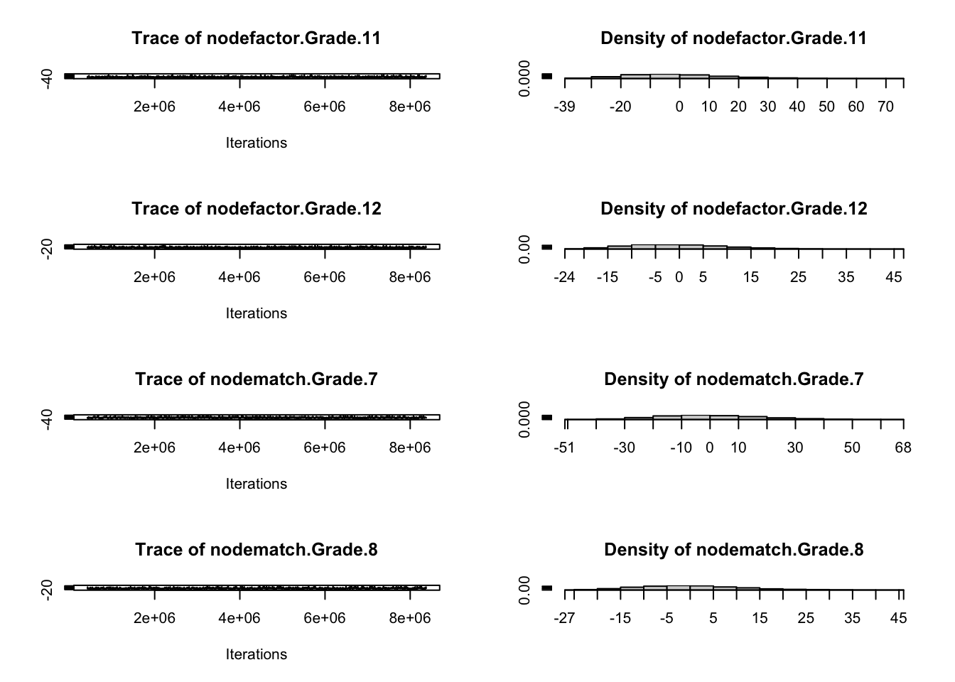
mcmc.diagnostics(fauxmodel.03)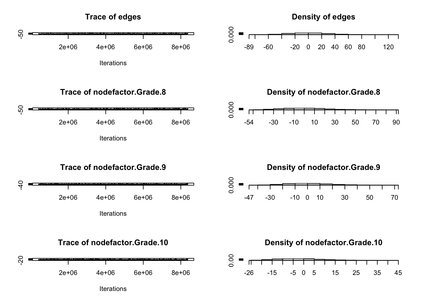
Sample statistics summary:
Iterations = 419840:8374272
Thinning interval = 2048
Number of chains = 1
Sample size per chain = 3885
1. Empirical mean and standard deviation for each variable,
plus standard error of the mean:
Mean SD Naive SE Time-series SE
edges 1.228829 26.897 0.43153 1.15438
nodefactor.Grade.8 1.630631 23.074 0.37020 1.07012
nodefactor.Grade.9 1.065894 17.346 0.27830 0.58519
nodefactor.Grade.10 -1.155212 10.785 0.17303 0.38619
nodefactor.Grade.11 -0.643243 16.635 0.26688 0.76166
nodefactor.Grade.12 0.091634 10.153 0.16290 0.41081
nodematch.Grade.7 0.747748 18.046 0.28953 0.82501
nodematch.Grade.8 0.891634 11.242 0.18037 0.52586
nodematch.Grade.9 0.499871 7.889 0.12657 0.27499
nodematch.Grade.10 -0.371171 4.282 0.06871 0.16097
nodematch.Grade.11 -0.225483 7.486 0.12010 0.35730
nodematch.Grade.12 0.182754 3.809 0.06110 0.16770
nodefactor.Race.Hisp 0.063835 28.108 0.45096 0.98508
nodefactor.Race.NatAm 1.927413 27.824 0.44640 1.20659
nodefactor.Race.Other -0.004118 1.051 0.01687 0.01850
nodefactor.Race.White 0.289318 11.229 0.18016 0.42369
nodematch.Race.Hisp 0.031918 10.810 0.17343 0.34321
nodematch.Race.NatAm 0.756242 10.819 0.17357 0.45768
nodematch.Race.White 0.051223 2.311 0.03707 0.08001
gwesp.fixed.0.25 1.563917 30.264 0.48555 1.29860
2. Quantiles for each variable:
2.5% 25% 50% 75% 97.5%
edges -48.00 -18.00 0.0000 19.00 56.00
nodefactor.Grade.8 -38.00 -15.00 0.0000 16.00 54.00
nodefactor.Grade.9 -29.00 -12.00 0.0000 12.00 38.00
nodefactor.Grade.10 -19.00 -9.00 -2.0000 5.00 23.00
nodefactor.Grade.11 -28.00 -13.00 -2.0000 10.00 36.90
nodefactor.Grade.12 -17.00 -7.00 -1.0000 7.00 22.00
nodematch.Grade.7 -31.00 -12.00 -1.0000 13.00 39.00
nodematch.Grade.8 -18.00 -7.00 0.0000 8.00 27.00
nodematch.Grade.9 -13.00 -5.00 0.0000 5.00 18.00
nodematch.Grade.10 -7.00 -4.00 -1.0000 2.00 9.00
nodematch.Grade.11 -12.00 -6.00 -1.0000 4.00 16.90
nodematch.Grade.12 -5.00 -3.00 0.0000 2.00 9.00
nodefactor.Race.Hisp -50.00 -20.00 -1.0000 18.00 59.00
nodefactor.Race.NatAm -48.00 -18.00 0.0000 20.00 61.00
nodefactor.Race.Other -1.00 -1.00 0.0000 1.00 3.00
nodefactor.Race.White -20.00 -8.00 -1.0000 8.00 24.00
nodematch.Race.Hisp -19.00 -7.00 -1.0000 7.00 23.00
nodematch.Race.NatAm -18.00 -7.00 0.0000 7.00 24.00
nodematch.Race.White -4.00 -2.00 0.0000 1.00 5.00
gwesp.fixed.0.25 -51.57 -20.09 0.1571 21.68 64.03
Are sample statistics significantly different from observed?
edges nodefactor.Grade.8 nodefactor.Grade.9 nodefactor.Grade.10
diff. 1.2288288 1.6306306 1.06589447 -1.155212355
test stat. 1.0644888 1.5237776 1.82143820 -2.991305231
P-val. 0.2871073 0.1275643 0.06854027 0.002777877
nodefactor.Grade.11 nodefactor.Grade.12 nodematch.Grade.7
diff. -0.6432432 0.09163449 0.7477477
test stat. -0.8445320 0.22305891 0.9063549
P-val. 0.3983722 0.82348966 0.3647480
nodematch.Grade.8 nodematch.Grade.9 nodematch.Grade.10
diff. 0.89163449 0.49987130 -0.37117117
test stat. 1.69557892 1.81779103 -2.30585463
P-val. 0.08996565 0.06909608 0.02111876
nodematch.Grade.11 nodematch.Grade.12 nodefactor.Race.Hisp
diff. -0.2254826 0.1827542 0.06383526
test stat. -0.6310693 1.0897886 0.06480240
P-val. 0.5279952 0.2758063 0.94833133
nodefactor.Race.NatAm nodefactor.Race.Other nodefactor.Race.White
diff. 1.9274131 -0.004118404 0.2893179
test stat. 1.5973991 -0.222589074 0.6828581
P-val. 0.1101768 0.823855341 0.4946965
nodematch.Race.Hisp nodematch.Race.NatAm nodematch.Race.White
diff. 0.03191763 0.75624196 0.05122265
test stat. 0.09299831 1.65235422 0.64023248
P-val. 0.92590490 0.09846236 0.52202147
gwesp.fixed.0.25 (Omni)
diff. 1.5639174 NA
test stat. 1.2043063 5.854200e+01
P-val. 0.2284712 2.018804e-05
Sample statistics cross-correlations:
edges nodefactor.Grade.8 nodefactor.Grade.9
edges 1.00000000 0.459964472 0.396886409
nodefactor.Grade.8 0.45996447 1.000000000 0.072626033
nodefactor.Grade.9 0.39688641 0.072626033 1.000000000
nodefactor.Grade.10 0.33276104 0.025927785 0.067633961
nodefactor.Grade.11 0.39272107 0.084576572 0.061769742
nodefactor.Grade.12 0.25320724 -0.059090616 0.112383398
nodematch.Grade.7 0.65026628 -0.018822401 -0.017715850
nodematch.Grade.8 0.44307879 0.989896818 0.062580579
nodematch.Grade.9 0.33745996 0.073289483 0.952690871
nodematch.Grade.10 0.24309670 0.017270715 -0.005417301
nodematch.Grade.11 0.34630038 0.085518086 0.025305141
nodematch.Grade.12 0.12540717 -0.088609373 0.025726423
nodefactor.Race.Hisp 0.78954179 0.263312571 0.307753742
nodefactor.Race.NatAm 0.76495588 0.460636104 0.329104164
nodefactor.Race.Other 0.05441431 -0.002058282 0.117238038
nodefactor.Race.White 0.58680550 0.144399864 0.118076268
nodematch.Race.Hisp 0.59455202 0.161300762 0.228716555
nodematch.Race.NatAm 0.59239418 0.384707258 0.269027966
nodematch.Race.White 0.27338989 0.046875625 0.001662936
gwesp.fixed.0.25 0.94627142 0.441880622 0.338635699
nodefactor.Grade.10 nodefactor.Grade.11
edges 0.332761042 0.39272107
nodefactor.Grade.8 0.025927785 0.08457657
nodefactor.Grade.9 0.067633961 0.06176974
nodefactor.Grade.10 1.000000000 0.13288816
nodefactor.Grade.11 0.132888159 1.00000000
nodefactor.Grade.12 0.169025161 0.11339637
nodematch.Grade.7 0.037084033 -0.03216177
nodematch.Grade.8 0.014524091 0.07394904
nodematch.Grade.9 -0.004843513 0.01718674
nodematch.Grade.10 0.887396642 0.05235392
nodematch.Grade.11 0.080293123 0.96100485
nodematch.Grade.12 0.053187403 0.02699531
nodefactor.Race.Hisp 0.225220686 0.23932454
nodefactor.Race.NatAm 0.203558094 0.30022969
nodefactor.Race.Other 0.058195377 0.02633650
nodefactor.Race.White 0.323295444 0.29102999
nodematch.Race.Hisp 0.148967462 0.12933411
nodematch.Race.NatAm 0.139809346 0.20455857
nodematch.Race.White 0.215520812 0.12977622
gwesp.fixed.0.25 0.270116122 0.36955772
nodefactor.Grade.12 nodematch.Grade.7 nodematch.Grade.8
edges 0.2532072351 0.65026628 0.443078794
nodefactor.Grade.8 -0.0590906165 -0.01882240 0.989896818
nodefactor.Grade.9 0.1123833976 -0.01771585 0.062580579
nodefactor.Grade.10 0.1690251609 0.03708403 0.014524091
nodefactor.Grade.11 0.1133963666 -0.03216177 0.073949042
nodefactor.Grade.12 1.0000000000 -0.02475757 -0.071281678
nodematch.Grade.7 -0.0247575698 1.00000000 -0.020604472
nodematch.Grade.8 -0.0712816778 -0.02060447 1.000000000
nodematch.Grade.9 0.0370417510 -0.01916616 0.070958470
nodematch.Grade.10 0.0440855332 0.05170277 0.016346951
nodematch.Grade.11 0.0584800338 -0.03432544 0.080690935
nodematch.Grade.12 0.8702715162 -0.04246067 -0.089115805
nodefactor.Race.Hisp 0.2429477826 0.61184083 0.246335714
nodefactor.Race.NatAm 0.1279697751 0.44927883 0.452843195
nodefactor.Race.Other 0.0295855861 -0.01136026 -0.002063883
nodefactor.Race.White 0.0793088393 0.47070908 0.133925246
nodematch.Race.Hisp 0.1759814879 0.51739548 0.148410266
nodematch.Race.NatAm 0.0770818153 0.34729239 0.382014444
nodematch.Race.White 0.0008314313 0.25139506 0.042196438
gwesp.fixed.0.25 0.2256984357 0.64972149 0.435940731
nodematch.Grade.9 nodematch.Grade.10 nodematch.Grade.11
edges 0.337459961 0.243096697 0.346300384
nodefactor.Grade.8 0.073289483 0.017270715 0.085518086
nodefactor.Grade.9 0.952690871 -0.005417301 0.025305141
nodefactor.Grade.10 -0.004843513 0.887396642 0.080293123
nodefactor.Grade.11 0.017186740 0.052353922 0.961004854
nodefactor.Grade.12 0.037041751 0.044085533 0.058480034
nodematch.Grade.7 -0.019166165 0.051702769 -0.034325441
nodematch.Grade.8 0.070958470 0.016346951 0.080690935
nodematch.Grade.9 1.000000000 -0.029677295 0.007750823
nodematch.Grade.10 -0.029677295 1.000000000 0.035207613
nodematch.Grade.11 0.007750823 0.035207613 1.000000000
nodematch.Grade.12 0.002742886 -0.001080840 0.012661445
nodefactor.Race.Hisp 0.258611554 0.144995748 0.199753179
nodefactor.Race.NatAm 0.295376831 0.162227304 0.271779087
nodefactor.Race.Other 0.106084905 0.029744061 0.020068735
nodefactor.Race.White 0.075566867 0.262126004 0.263692013
nodematch.Race.Hisp 0.195380146 0.090007493 0.101771895
nodematch.Race.NatAm 0.248660861 0.117764249 0.184302809
nodematch.Race.White -0.020499954 0.190529095 0.111552806
gwesp.fixed.0.25 0.300795942 0.204436631 0.341460574
nodematch.Grade.12 nodefactor.Race.Hisp
edges 0.125407172 0.78954179
nodefactor.Grade.8 -0.088609373 0.26331257
nodefactor.Grade.9 0.025726423 0.30775374
nodefactor.Grade.10 0.053187403 0.22522069
nodefactor.Grade.11 0.026995310 0.23932454
nodefactor.Grade.12 0.870271516 0.24294778
nodematch.Grade.7 -0.042460667 0.61184083
nodematch.Grade.8 -0.089115805 0.24633571
nodematch.Grade.9 0.002742886 0.25861155
nodematch.Grade.10 -0.001080840 0.14499575
nodematch.Grade.11 0.012661445 0.19975318
nodematch.Grade.12 1.000000000 0.14699245
nodefactor.Race.Hisp 0.146992451 1.00000000
nodefactor.Race.NatAm 0.040818644 0.28244406
nodefactor.Race.Other 0.020316764 0.03188367
nodefactor.Race.White 0.002170744 0.38212316
nodematch.Race.Hisp 0.112320633 0.91130374
nodematch.Race.NatAm 0.015071879 0.12365431
nodematch.Race.White -0.027247572 0.14370950
gwesp.fixed.0.25 0.124397646 0.72007172
nodefactor.Race.NatAm nodefactor.Race.Other
edges 0.76495588 0.0544143094
nodefactor.Grade.8 0.46063610 -0.0020582818
nodefactor.Grade.9 0.32910416 0.1172380382
nodefactor.Grade.10 0.20355809 0.0581953769
nodefactor.Grade.11 0.30022969 0.0263365030
nodefactor.Grade.12 0.12796978 0.0295855861
nodematch.Grade.7 0.44927883 -0.0113602626
nodematch.Grade.8 0.45284319 -0.0020638830
nodematch.Grade.9 0.29537683 0.1060849051
nodematch.Grade.10 0.16222730 0.0297440605
nodematch.Grade.11 0.27177909 0.0200687350
nodematch.Grade.12 0.04081864 0.0203167639
nodefactor.Race.Hisp 0.28244406 0.0318836674
nodefactor.Race.NatAm 1.00000000 0.0195491353
nodefactor.Race.Other 0.01954914 1.0000000000
nodefactor.Race.White 0.27706503 0.0180514784
nodematch.Race.Hisp 0.10756829 0.0183418333
nodematch.Race.NatAm 0.92171447 0.0091030491
nodematch.Race.White 0.08739136 0.0001928628
gwesp.fixed.0.25 0.74419089 0.0258951105
nodefactor.Race.White nodematch.Race.Hisp
edges 0.586805498 0.59455202
nodefactor.Grade.8 0.144399864 0.16130076
nodefactor.Grade.9 0.118076268 0.22871655
nodefactor.Grade.10 0.323295444 0.14896746
nodefactor.Grade.11 0.291029992 0.12933411
nodefactor.Grade.12 0.079308839 0.17598149
nodematch.Grade.7 0.470709080 0.51739548
nodematch.Grade.8 0.133925246 0.14841027
nodematch.Grade.9 0.075566867 0.19538015
nodematch.Grade.10 0.262126004 0.09000749
nodematch.Grade.11 0.263692013 0.10177190
nodematch.Grade.12 0.002170744 0.11232063
nodefactor.Race.Hisp 0.382123163 0.91130374
nodefactor.Race.NatAm 0.277065035 0.10756829
nodefactor.Race.Other 0.018051478 0.01834183
nodefactor.Race.White 1.000000000 0.21158740
nodematch.Race.Hisp 0.211587400 1.00000000
nodematch.Race.NatAm 0.137259814 0.04098433
nodematch.Race.White 0.682895526 0.09059960
gwesp.fixed.0.25 0.567496798 0.53471340
nodematch.Race.NatAm nodematch.Race.White
edges 0.592394176 0.2733898917
nodefactor.Grade.8 0.384707258 0.0468756251
nodefactor.Grade.9 0.269027966 0.0016629361
nodefactor.Grade.10 0.139809346 0.2155208120
nodefactor.Grade.11 0.204558574 0.1297762155
nodefactor.Grade.12 0.077081815 0.0008314313
nodematch.Grade.7 0.347292394 0.2513950614
nodematch.Grade.8 0.382014444 0.0421964380
nodematch.Grade.9 0.248660861 -0.0204999543
nodematch.Grade.10 0.117764249 0.1905290952
nodematch.Grade.11 0.184302809 0.1115528060
nodematch.Grade.12 0.015071879 -0.0272475723
nodefactor.Race.Hisp 0.123654309 0.1437094980
nodefactor.Race.NatAm 0.921714466 0.0873913599
nodefactor.Race.Other 0.009103049 0.0001928628
nodefactor.Race.White 0.137259814 0.6828955255
nodematch.Race.Hisp 0.040984326 0.0905996044
nodematch.Race.NatAm 1.000000000 0.0394188258
nodematch.Race.White 0.039418826 1.0000000000
gwesp.fixed.0.25 0.588878771 0.2675217932
gwesp.fixed.0.25
edges 0.94627142
nodefactor.Grade.8 0.44188062
nodefactor.Grade.9 0.33863570
nodefactor.Grade.10 0.27011612
nodefactor.Grade.11 0.36955772
nodefactor.Grade.12 0.22569844
nodematch.Grade.7 0.64972149
nodematch.Grade.8 0.43594073
nodematch.Grade.9 0.30079594
nodematch.Grade.10 0.20443663
nodematch.Grade.11 0.34146057
nodematch.Grade.12 0.12439765
nodefactor.Race.Hisp 0.72007172
nodefactor.Race.NatAm 0.74419089
nodefactor.Race.Other 0.02589511
nodefactor.Race.White 0.56749680
nodematch.Race.Hisp 0.53471340
nodematch.Race.NatAm 0.58887877
nodematch.Race.White 0.26752179
gwesp.fixed.0.25 1.00000000
Sample statistics auto-correlation:
Chain 1
edges nodefactor.Grade.8 nodefactor.Grade.9 nodefactor.Grade.10
Lag 0 1.0000000 1.0000000 1.0000000 1.0000000
Lag 2048 0.6969872 0.7384123 0.5967802 0.5330776
Lag 4096 0.5207419 0.5677893 0.3914377 0.3673704
Lag 6144 0.4133212 0.4529588 0.2622251 0.2709906
Lag 8192 0.3171991 0.3698514 0.1886247 0.2111878
Lag 10240 0.2405876 0.2938766 0.1412652 0.1504430
nodefactor.Grade.11 nodefactor.Grade.12 nodematch.Grade.7
Lag 0 1.0000000 1.0000000 1.0000000
Lag 2048 0.7341227 0.6752044 0.7431929
Lag 4096 0.5675207 0.5125547 0.5727706
Lag 6144 0.4586239 0.3849823 0.4560739
Lag 8192 0.3737213 0.3007942 0.3507952
Lag 10240 0.3041538 0.2427691 0.2842608
nodematch.Grade.8 nodematch.Grade.9 nodematch.Grade.10
Lag 0 1.0000000 1.0000000 1.0000000
Lag 2048 0.7485853 0.6169299 0.5657269
Lag 4096 0.5771761 0.4150335 0.3870280
Lag 6144 0.4612042 0.2791780 0.2799626
Lag 8192 0.3763141 0.2042605 0.2166732
Lag 10240 0.3013863 0.1582886 0.1611194
nodematch.Grade.11 nodematch.Grade.12 nodefactor.Race.Hisp
Lag 0 1.0000000 1.0000000 1.0000000
Lag 2048 0.7685645 0.7510663 0.6065833
Lag 4096 0.6013098 0.5788866 0.3939291
Lag 6144 0.4893380 0.4472638 0.2769766
Lag 8192 0.3971572 0.3417641 0.1801089
Lag 10240 0.3214253 0.2595685 0.1265056
nodefactor.Race.NatAm nodefactor.Race.Other nodefactor.Race.White
Lag 0 1.0000000 1.000000000 1.0000000
Lag 2048 0.7058863 0.092249778 0.6337069
Lag 4096 0.5353234 0.007672521 0.4448835
Lag 6144 0.4225623 -0.025177886 0.3280192
Lag 8192 0.3235451 0.021421148 0.2373814
Lag 10240 0.2419023 0.003243681 0.1790955
nodematch.Race.Hisp nodematch.Race.NatAm nodematch.Race.White
Lag 0 1.00000000 1.0000000 1.0000000
Lag 2048 0.54657891 0.7009725 0.5639525
Lag 4096 0.32497045 0.5298580 0.3582003
Lag 6144 0.21331983 0.4085585 0.2484061
Lag 8192 0.13353998 0.3124094 0.1767961
Lag 10240 0.09522135 0.2299103 0.1272778
gwesp.fixed.0.25
Lag 0 1.0000000
Lag 2048 0.6835525
Lag 4096 0.5239579
Lag 6144 0.4142536
Lag 8192 0.3179093
Lag 10240 0.2391275
Sample statistics burn-in diagnostic (Geweke):
Chain 1
Fraction in 1st window = 0.1
Fraction in 2nd window = 0.5
edges nodefactor.Grade.8 nodefactor.Grade.9
-0.08452458 -1.82528519 0.90687970
nodefactor.Grade.10 nodefactor.Grade.11 nodefactor.Grade.12
-0.02432314 -1.03287990 2.09986213
nodematch.Grade.7 nodematch.Grade.8 nodematch.Grade.9
0.34912052 -1.82845621 0.54997480
nodematch.Grade.10 nodematch.Grade.11 nodematch.Grade.12
-0.52100539 -1.08159933 1.96178082
nodefactor.Race.Hisp nodefactor.Race.NatAm nodefactor.Race.Other
0.34269430 -0.64134408 0.57787126
nodefactor.Race.White nodematch.Race.Hisp nodematch.Race.NatAm
-0.15663203 0.21823417 -0.82060767
nodematch.Race.White gwesp.fixed.0.25
-0.45066360 -0.12038549
Individual P-values (lower = worse):
edges nodefactor.Grade.8 nodefactor.Grade.9
0.93263936 0.06795800 0.36447042
nodefactor.Grade.10 nodefactor.Grade.11 nodefactor.Grade.12
0.98059486 0.30166010 0.03574097
nodematch.Grade.7 nodematch.Grade.8 nodematch.Grade.9
0.72699883 0.06748111 0.58233666
nodematch.Grade.10 nodematch.Grade.11 nodematch.Grade.12
0.60236301 0.27943060 0.04978801
nodefactor.Race.Hisp nodefactor.Race.NatAm nodefactor.Race.Other
0.73182845 0.52129915 0.56335104
nodefactor.Race.White nodematch.Race.Hisp nodematch.Race.NatAm
0.87553486 0.82724666 0.41186978
nodematch.Race.White gwesp.fixed.0.25
0.65223202 0.90417779
Joint P-value (lower = worse): 0.4810945
Note: MCMC diagnostics shown here are from the last round of
simulation, prior to computation of final parameter estimates.
Because the final estimates are refinements of those used for this
simulation run, these diagnostics may understate model performance.
To directly assess the performance of the final model on in-model
statistics, please use the GOF command: gof(ergmFitObject,
GOF=~model).GOF: Model 3
fauxmodel.03.gof <- gof(fauxmodel.03)
plot(fauxmodel.03.gof)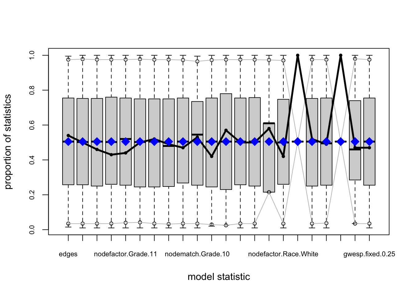
BERGMs
The ERGM section treats \(\theta\) as fixed and returns a point estimate \(\hat\theta\) (via MLE or MCMLE). A Bayesian exponential random graph model (BERGM) keeps the same likelihood,
\[ \Pr(Y = y_{\text{obs}} \mid \theta) = \frac{\exp\{\theta^\top g(y_{\text{obs}})\}}{k(\theta)}, \]
but places a prior \(p(\theta)\) on the parameters and targets the posterior
\[ p(\theta \mid Y = y_{\text{obs}}) \;=\; \frac{\Pr(Y = y_{\text{obs}} \mid \theta)\, p(\theta)}{\int \Pr(Y = y_{\text{obs}} \mid \theta')\, p(\theta')\, d\theta'}. \]
The sufficient statistics \(g(y)\), the change statistics \(\delta_{ij}(y)\), and the interpretation of each \(\theta_k\) is unchanged. What’s changed is our inferential goal, shifting from a single \(\hat\theta\) to a distribution for \(\theta\).
Handwavy details
See Bayesian perspectives on exponential random graph models, a recent (May 2026) survey for BERGMs. In short, the Bayesian approach helps regularize coefficients toward modest values, while also enabling principled uncertainty quantification (i.e., posterior credible intervals). However, the problem is now doubly-intractable: each evaluation of \(\Pr(Y = y_{\text{obs}} \mid \theta)\) requires the normalizing constant \(k(\theta)\) from before, but now \(\theta\) itself is unknown. The Bergm package uses an exchange algorithm: at each step it simulates an auxiliary network at a proposed \(\theta\) (via ergm’s MCMC) and accepts or rejects that proposal by comparing auxiliary and observed sufficient statistics, avoiding explicit evaluation of \(k(\theta)\). This inner network simulation is one more layer of MCMC nested inside the outer sampler over \(\theta\).
To move \(\theta\), bergm() runs parallel adaptive direction sampling (PADS) across several \(\theta\)-chains (by default, twice the number of model terms). Each step proposes a new value for chain \(h\) by
\[ \theta^{\text{prop}} \;=\; \theta_h \;+\; \gamma\,(\theta_{h_1} - \theta_{h_2}) \;+\; \varepsilon, \qquad \varepsilon \sim N(0,\, V_{\text{proposal}}\, I), \]
where \(h_1, h_2\) are two other chains chosen at random; the exchange algorithm then decides whether to accept \(\theta^{\text{prop}}\).
gammascales the directional step along their difference.V.proposalsets the variance of the extra random jitter.
Together, these parameters control proposal size. We can tune them (along with burn.in and main.iters) until we have a reasonable acceptance rate (\(~20\%\)). See the documentation for syntax. As before, we’ll need to make sure to check diagnostics before interpreting coefficients.
Diagnostics
The standard Bergm workflow has three steps after fitting:
summary()reports the acceptance rate in the exchange algorithm (a good value is \(~20\%\)), posterior means, standard deviations, and credible intervals in the form of posterior percentiles (e.g., \(95\%\) credible interval is bewteen2.5%and97.5%). It also reports two standard errors for each \(\theta_k\):Naive SEtreats the \(n\) posterior draws as independent, ignoring MCMC autocorrelation and typically underestimates uncertainty when the chain mixes slowly.Time-series SEaccounts for autocorrelation in the draws. IfTime-series SEis much larger thanNaive SE, this is a signal that the chain is mixing poorly for that parameter and the credible intervals may be too narrow.
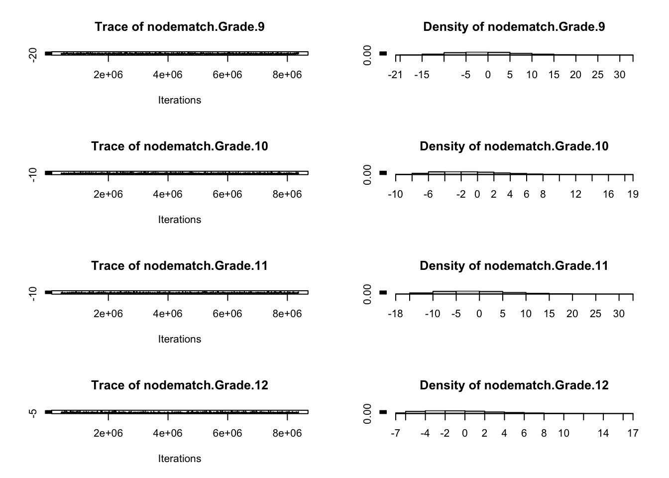
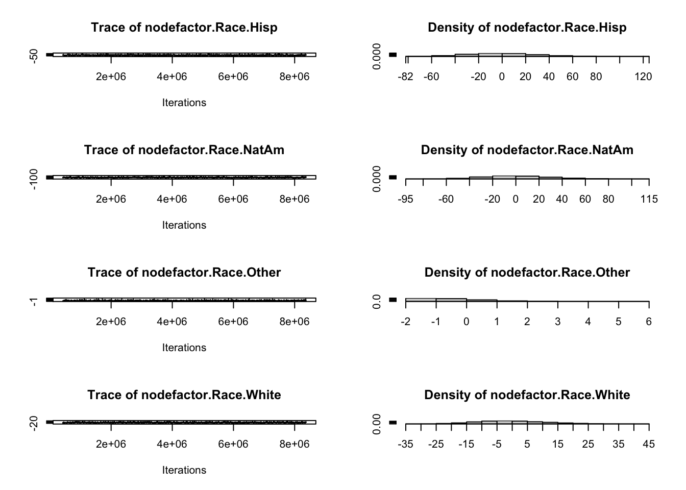
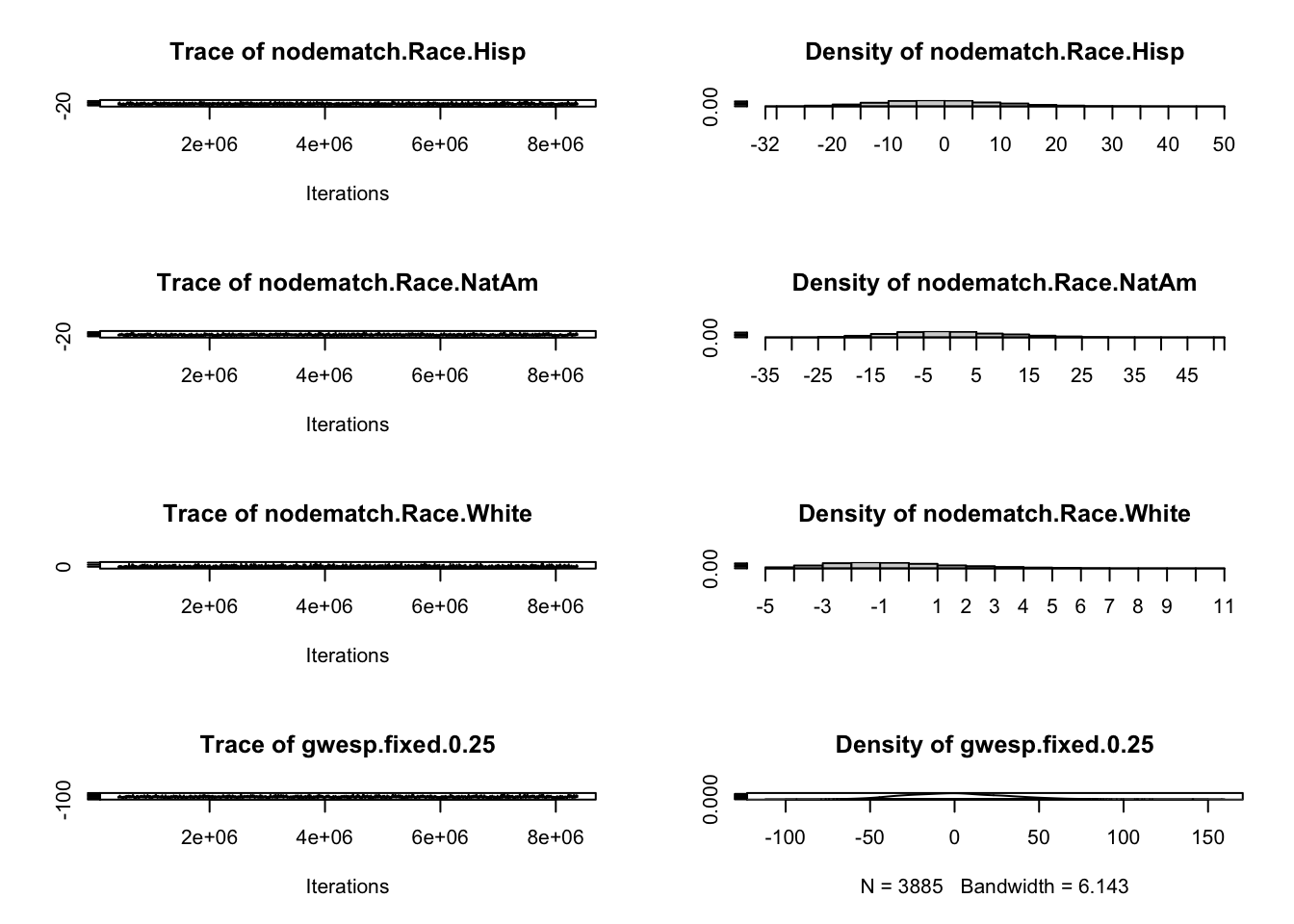
plot()shows three panels per parameter: marginal posterior density (left), trace plot (middle), and autocorrelation (right).- Density: should look reasonably smooth and stable across MCMC pages; sharp spikes or multi-modality can indicate poor mixing or label-switching-like behavior.
- Trace: should look stationary.
- Autocorrelation: should decay quickly toward zero as lag increases. Slow decay means successive draws are highly dependent and effective sample size is small.
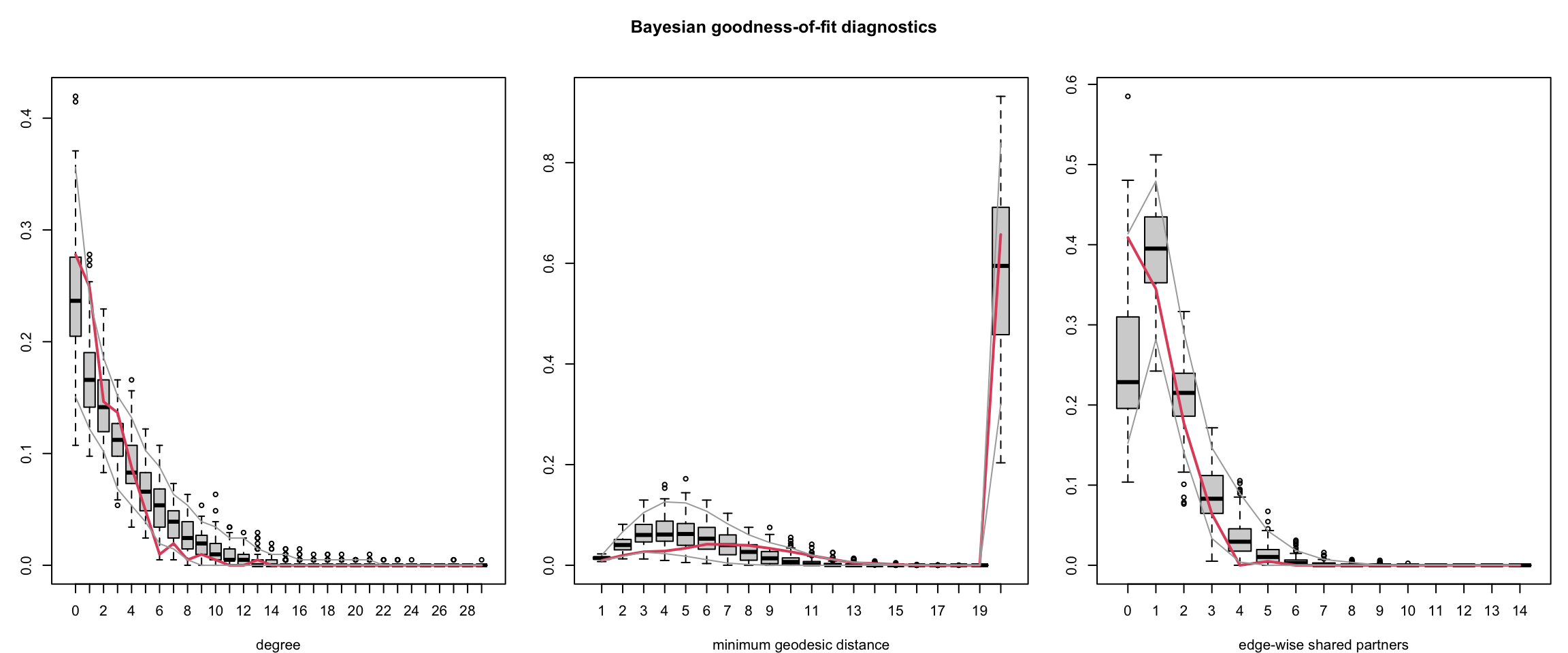
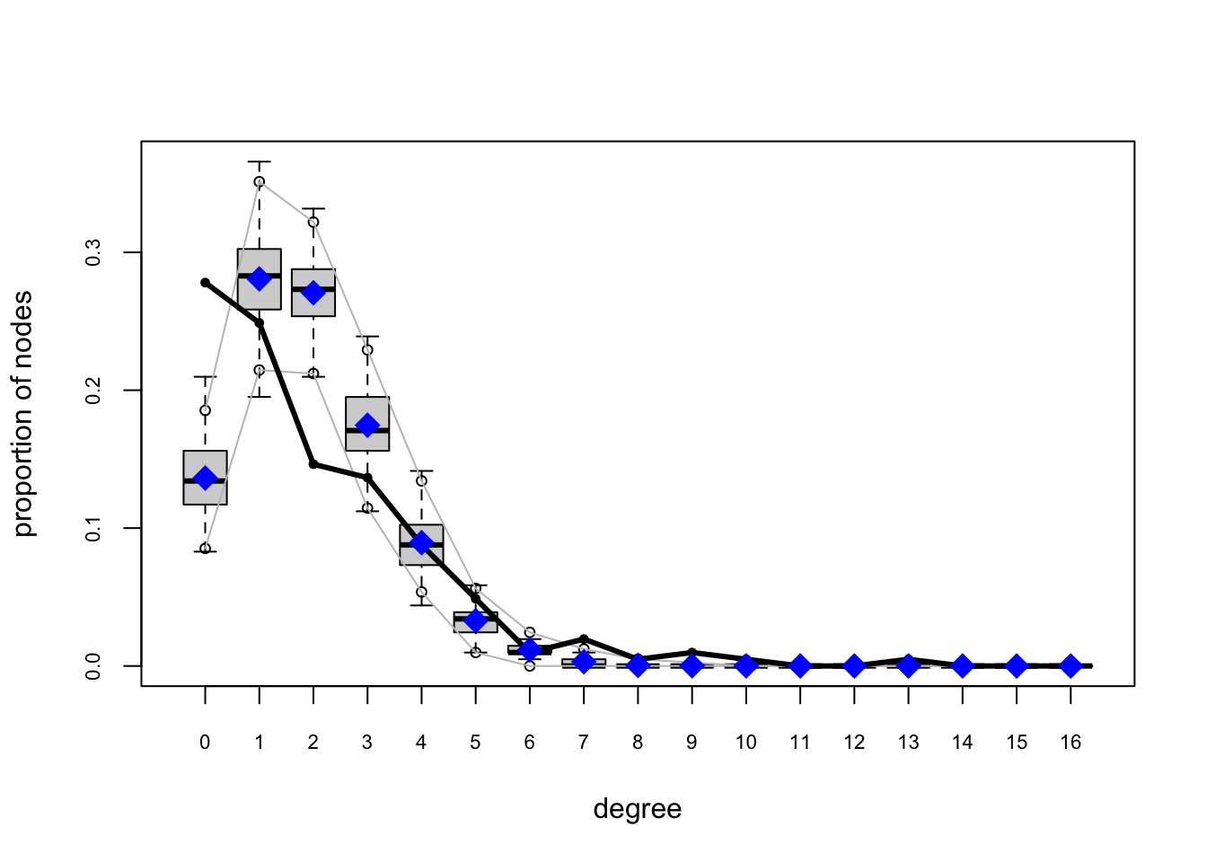
bgof()carries out Bayesian GOF: it draws \(\theta\) from the posterior, simulates networks at each draw, and compares degree, minimum geodesic distance and edgewise shared partner distributions to \(y_{\text{obs}}\). The red line is \(y_{\text{obs}}\); boxplots summarize the posterior predictive simulations; gray lines mark the \(5\%\) and \(95\%\) simulation quantiles at each bin.
Implementing BERGM
We fit the same formula as Model 3. Recall that the frequentist methods fit fixed some race homophily coefficients at \(-\infty\). By default, the bergm() function initializes MPLE coefficients, and \(-\infty\) starting values break the exchange algorithm. We will instead manually specify the initialization bergm_start, replacing \(-\infty\) entries with a large negative value.
With default values, the acceptance rate is only \(\sim 3\%\) (poor mixing). A few quick tests found the parameters below, though they can probably still be tuned more.
bergm_start <- coef(fauxmodel.03)
bergm_start[!is.finite(bergm_start)] <- -10

fauxmodel.bergm <- bergm(
  mesa ~ edges +
    nodefactor("Grade") + nodematch("Grade", diff = TRUE) +
    nodefactor("Race") + nodematch("Race", diff = TRUE) +
    gwesp(0.25, fixed = TRUE),
  startVals  = bergm_start,
  burn.in    = 200,
  main.iters = 2000,
  aux.iters  = 1000,
  gamma      = 0.30,
  V.proposal = 0.0005
)
summary(fauxmodel.bergm)
 Posterior Density Estimate for Model: y ~ edges + nodefactor("Grade") + nodematch("Grade", diff = TRUE) + nodefactor("Race") + nodematch("Race", diff = TRUE) + gwesp(0.25, fixed = TRUE)

                                      Mean        SD     Naive SE
theta1 (edges)                  -8.3216258 1.5976965 0.0053858339
theta2 (nodefactor.Grade.8)      1.1590616 0.7759647 0.0026157763
theta3 (nodefactor.Grade.9)      2.2525447 0.7941709 0.0026771495
theta4 (nodefactor.Grade.10)     2.4049757 0.7596920 0.0025609213
theta5 (nodefactor.Grade.11)     2.2403934 0.7785829 0.0026246026
theta6 (nodefactor.Grade.12)     2.8405935 0.8229257 0.0027740819
theta7 (nodematch.Grade.7)       6.2320911 1.3778713 0.0046448031
theta8 (nodematch.Grade.8)       3.8076558 0.9421662 0.0031760415
theta9 (nodematch.Grade.9)       1.8235596 0.7920156 0.0026698839
theta10 (nodematch.Grade.10)     1.5641907 0.8996292 0.0030326495
theta11 (nodematch.Grade.11)     2.1765454 0.8603155 0.0029001228
theta12 (nodematch.Grade.12)     1.1879359 1.1337038 0.0038217146
theta13 (nodefactor.Race.Hisp)  -1.2814838 0.4664444 0.0015723838
theta14 (nodefactor.Race.NatAm) -1.3321152 0.5046209 0.0017010767
theta15 (nodefactor.Race.Other) -3.2553423 1.7653958 0.0059511481
theta16 (nodefactor.Race.White) -0.8297547 0.5029666 0.0016955001
theta17 (nodematch.Race.Black)  -8.4298004 7.3942234 0.0249259220
theta18 (nodematch.Race.Hisp)    0.5745054 0.5403531 0.0018215299
theta19 (nodematch.Race.NatAm)   1.3961492 0.6081519 0.0020500798
theta20 (nodematch.Race.Other)  -3.3219371 9.9366660 0.0334964942
theta21 (nodematch.Race.White)   0.4653568 1.2136125 0.0040910870
theta22 (gwesp.fixed.0.25)       1.3489984 0.1419574 0.0004785383
                                Time-series SE
theta1 (edges)                     0.072434409
theta2 (nodefactor.Grade.8)        0.035598839
theta3 (nodefactor.Grade.9)        0.039019759
theta4 (nodefactor.Grade.10)       0.034077621
theta5 (nodefactor.Grade.11)       0.033632623
theta6 (nodefactor.Grade.12)       0.038599014
theta7 (nodematch.Grade.7)         0.066886233
theta8 (nodematch.Grade.8)         0.040821528
theta9 (nodematch.Grade.9)         0.034524682
theta10 (nodematch.Grade.10)       0.038560274
theta11 (nodematch.Grade.11)       0.036711137
theta12 (nodematch.Grade.12)       0.049116358
theta13 (nodefactor.Race.Hisp)     0.019616748
theta14 (nodefactor.Race.NatAm)    0.021672964
theta15 (nodefactor.Race.Other)    0.079456527
theta16 (nodefactor.Race.White)    0.021346645
theta17 (nodematch.Race.Black)     0.324556446
theta18 (nodematch.Race.Hisp)      0.023502973
theta19 (nodematch.Race.NatAm)     0.026111446
theta20 (nodematch.Race.Other)     0.455969673
theta21 (nodematch.Race.White)     0.052465957
theta22 (gwesp.fixed.0.25)         0.005871585

                                       2.5%         25%        50%        75%
theta1 (edges)                  -11.8347420  -9.2710155 -8.2239198 -7.2061058
theta2 (nodefactor.Grade.8)      -0.3423904   0.6429124  1.1507994  1.6305273
theta3 (nodefactor.Grade.9)       0.8969718   1.7017497  2.1863462  2.7174295
theta4 (nodefactor.Grade.10)      1.0196059   1.8794822  2.3914292  2.8859828
theta5 (nodefactor.Grade.11)      0.8532294   1.7131658  2.1954206  2.7154242
theta6 (nodefactor.Grade.12)      1.3413768   2.2790169  2.7959817  3.3610368
theta7 (nodematch.Grade.7)        3.8751030   5.2772659  6.1124505  7.0506594
theta8 (nodematch.Grade.8)        2.0594238   3.1659204  3.7649077  4.3912058
theta9 (nodematch.Grade.9)        0.3282604   1.2916004  1.8029497  2.3492940
theta10 (nodematch.Grade.10)     -0.1585349   0.9533592  1.5576182  2.1485756
theta11 (nodematch.Grade.11)      0.5393587   1.6132694  2.1501634  2.7305768
theta12 (nodematch.Grade.12)     -0.9987875   0.3944025  1.2098459  1.9644430
theta13 (nodefactor.Race.Hisp)   -2.2040103  -1.6017998 -1.2797301 -0.9626968
theta14 (nodefactor.Race.NatAm)  -2.3038592  -1.6755494 -1.3381818 -0.9875575
theta15 (nodefactor.Race.Other)  -7.5211859  -4.1100826 -2.9805202 -2.0210318
theta16 (nodefactor.Race.White)  -1.7933681  -1.1763508 -0.8395391 -0.4998877
theta17 (nodematch.Race.Black)  -24.6706223 -12.8152600 -8.0321003 -3.2096067
theta18 (nodematch.Race.Hisp)    -0.4828992   0.2071264  0.5719879  0.9350083
theta19 (nodematch.Race.NatAm)    0.2262771   0.9788389  1.3970305  1.8167941
theta20 (nodematch.Race.Other)  -22.5516091  -9.7613770 -3.5511470  3.2545337
theta21 (nodematch.Race.White)   -1.9486782  -0.3344216  0.4828976  1.3193588
theta22 (gwesp.fixed.0.25)        1.0665623   1.2543835  1.3494183  1.4451528
                                     97.5%
theta1 (edges)                  -5.4974050
theta2 (nodefactor.Grade.8)      2.7814623
theta3 (nodefactor.Grade.9)      3.9733795
theta4 (nodefactor.Grade.10)     3.9812610
theta5 (nodefactor.Grade.11)     3.8894899
theta6 (nodefactor.Grade.12)     4.5802147
theta7 (nodematch.Grade.7)       9.2742829
theta8 (nodematch.Grade.8)       5.7740764
theta9 (nodematch.Grade.9)       3.4481336
theta10 (nodematch.Grade.10)     3.3470215
theta11 (nodematch.Grade.11)     3.9489046
theta12 (nodematch.Grade.12)     3.3573524
theta13 (nodefactor.Race.Hisp)  -0.3833634
theta14 (nodefactor.Race.NatAm) -0.3370849
theta15 (nodefactor.Race.Other) -0.6941067
theta16 (nodefactor.Race.White)  0.1841097
theta17 (nodematch.Race.Black)   4.5485955
theta18 (nodematch.Race.Hisp)    1.6556552
theta19 (nodematch.Race.NatAm)   2.5848217
theta20 (nodematch.Race.Other)  16.6019259
theta21 (nodematch.Race.White)   2.7202056
theta22 (gwesp.fixed.0.25)       1.6263442

 Acceptance rate: 0.15
# plot(fauxmodel.bergm) works interactively but calls new graphics devices internally that Quarto cannot render....
plot(fauxmodel.bergm)bgof(
fauxmodel.bergm,
n.deg = 30, # degree bins
n.dist = 20, # distance bins
n.esp = 15 # edgewise shared partner bins
)